Vector Algebra on Linux with Python Script: Part 1
On this page
In this tutorial, we will discuss the vector algebra and corresponding calculations under Scientific Linux. For our purpose, I have chosen Python as the programming language for its simplicity and power of calculation. Any Linux distribution has by default a Python editor / compiler which is invoked through a terminal window. Let's go over some concepts of vector algebra.
Note: we only going to work on real space of two or three dimensions.
Vector Algebra
The Element of a vector space, from a mathematical point of view, can be represented as the array of a number of elements that belong to that vector space. More specifically, and in numerical computing approach, it can be represented as a list of real numbers, which has three basic characteristics:
Magnitude
The size of the vector and is represented with  ;this is the scalar part of a vector. For calculating the magnitude of a vector we have to perform the next formula:
X, Y and Z are the vector coordinates.
Direction
The direction of a vector is given by a directrix line having a specific angle for each axis of the coordinate system called director angles.
Where alpha, beta and gamma are the vector director angles and their cosines are the director cosines, they also can be calculated by dividing each vector coordinate by its magnitude.
Orientation
One of the two possible orientations between the same direction.
Vector Algebraic Sum
To make an algebraic sum of vectors, we must add the homologous coordinates of two vectors, attending the same properties of the algebraic sum of real numbers. Just as follows:

Product of a vector by a scalar
Given a vector and a scalar, product vector by a scalar is defined as the scalar product of each coordinate of the vector:
Where 
Unit Vector
A direct application for Product vector by a scalar is the unit vector, a unit vector is a normed vector of length 1.
Linear Combination
When we mix the past operations, algebraic sum and product vector-scalar, we obtain a linear combination, in which the result is also a vector belonging to the same vector space, as is:

Where vector A is a linear combination of vectors B and C.
Python on Scientific Linux 7.1
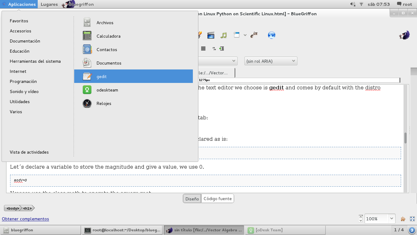
To implement vector algebra we chose Python as a calculus language. The text editor we choose is gedit and comes by default with the distro Scientific Linux 7.1.
Magnitude of a vector
Let´s call gedit using a terminal or just click on the icon at applications tab:
First we must work with lists, as representing vectors and should be declared as is:
V=[2, 2, 1]
Let´s declare a variable to store the magnitude and give a value, we use 0.
modV=0
Now we use the class math to operate the square root:
import math
The calculation of the magnitude:
modV=math.sqrt(V[0]**2+V[1]**2+V[2]**2)
As we can see, we have to use sub-index to indicate the item from the list that we will operate, starting from 0.
The complete script is the following:
V=[2, 2, 1]
modV=0
import math
modV=math.sqrt(V[0]**2+V[1]**2+V[2]**2)
print (modV)
Once finished we have to save the file with the extension .py and the locate the file path and open a terminal window there with right click and then "open in terminal window". After we have to call the python interpreter typing:
$ python [path]/yourfilename.py
this will open a window like this and give the result: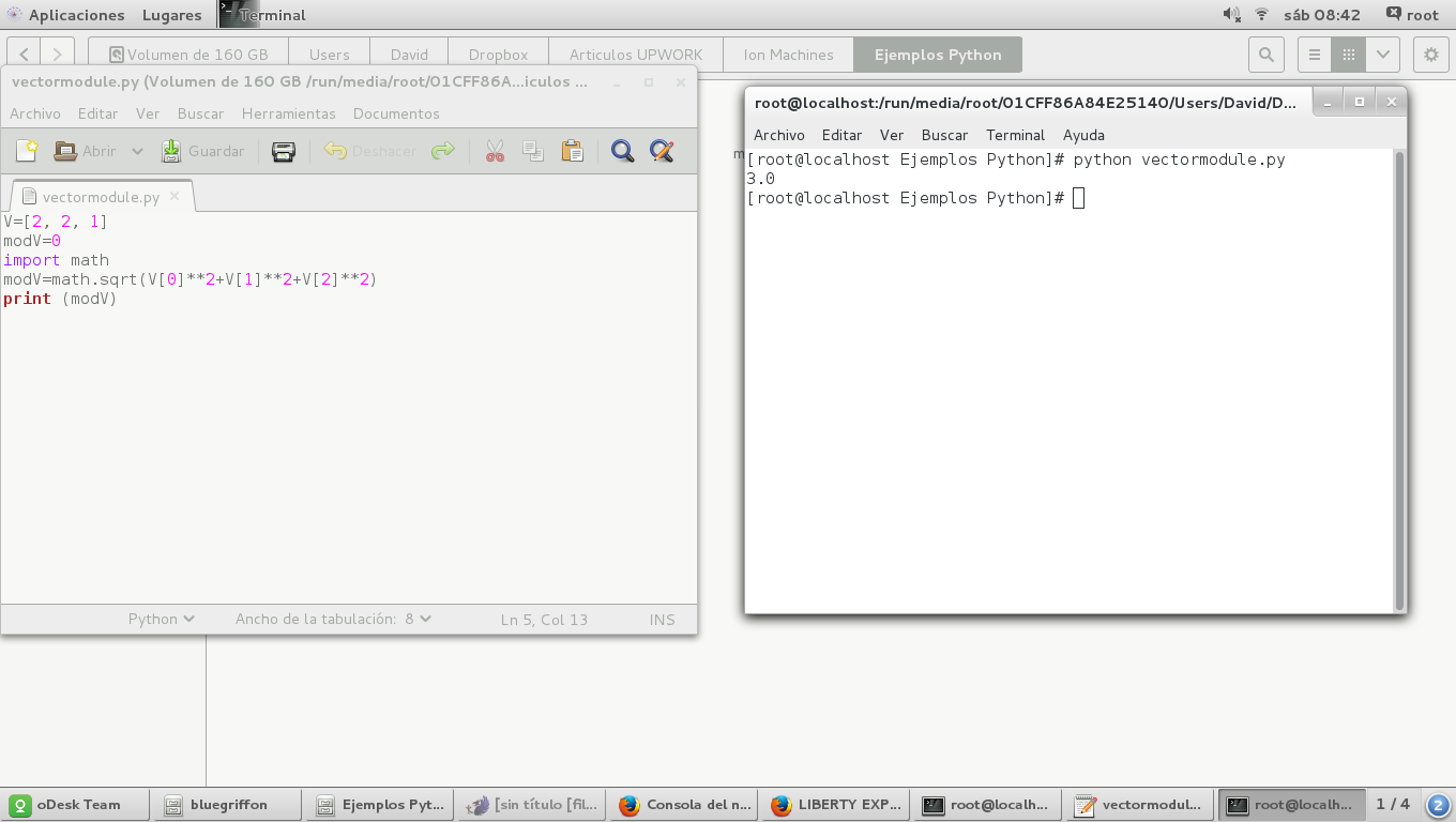
Another way to do it is using a for loop like these:
for x in range (0,3):
    modV+=V[x]**2
modV=math.sqrt(modV)
Here we have to use indentation techniques since python interpreter works in that way.
Direction of a vector
Use the class math
V=[2, 1, 2]
modV=0
import math
for x in range (0,3): #loop for calculating the magnitude
modV+=V[x]**2
modV=math.sqrt(modV)
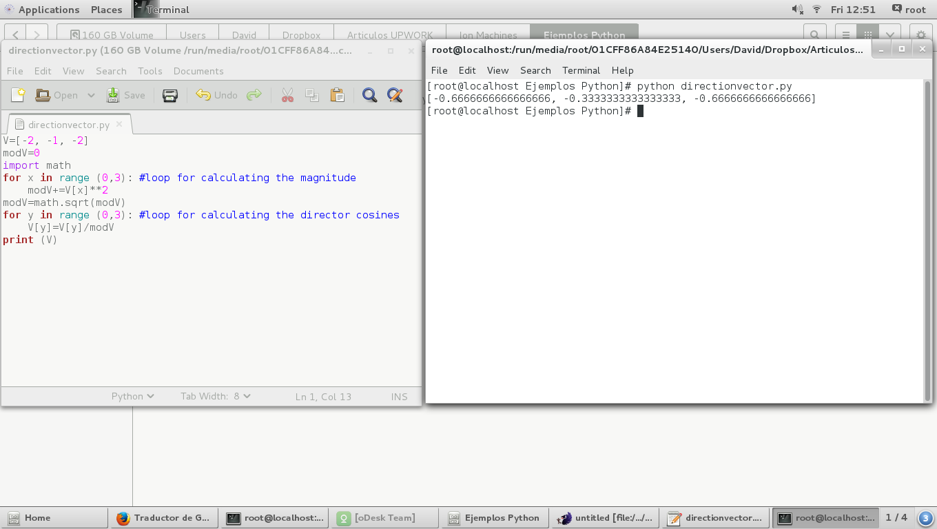
for y in range (0,3): #loop for calculating the director cosines
V[y]=V[y]/modV
print (V)
The result is the next: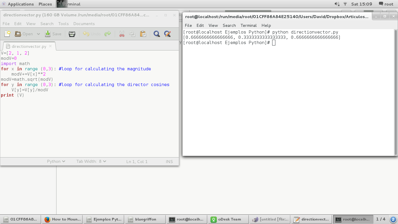
Another way to do it is using the trigonometric functions of math class, just like this:
First let´s calculate the director angles:
V=[2, 1, 2]
angles=[0,0,0]
modV=0
import math
for y in range (0,3): #loop for calculating the director angles in degrees
    angles[y]=math.degrees(math.acos(V[y]/modV))
And then let´s calculate the director cosines and print them
for z in range(0,3):    #loop for calculating the director cosines
    V[z]=math.cos(math.radians(angles[z]))
print (angles)
print (V)
And the result: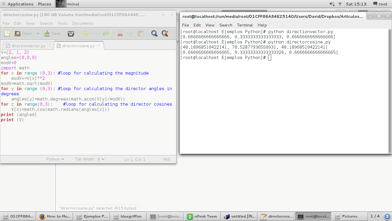
We can observe that the director cosines are the same value
Orientation of a vector
If we change the sign of all coordinates of a vector we, inherently, are changing the orientation of the vector, as is:
V=[-2, -1, -2]
angles=[0,0,0]
modV=0
import math
for y in range (0,3): #loop for calculating the director angles in degrees
    angles[y]=math.degrees(math.acos(V[y]/modV))for z in range(0,3):    #loop for calculating the director cosines
    V[z]=math.cos(math.radians(angles[z]))
print (angles)
print (V)
In the next image we can see the director angles are different in 180 degrees from the originals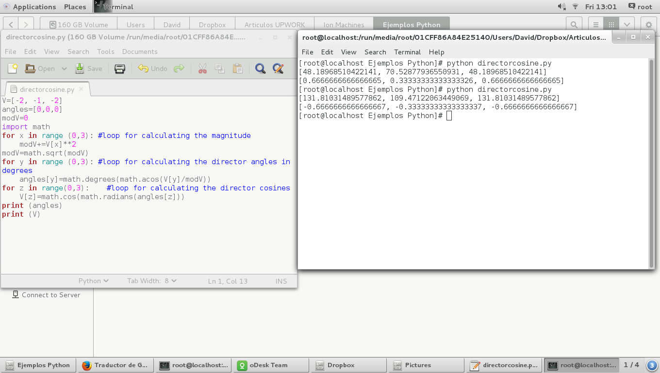
Vector Algebraic Sum
First we have to declare all vectors involved in algebraic sum, as is:
A=[1,2,4]
B=[2,1,4]
S=[0,0,0]
where we're going to sum A plus B and the result will store in S
Adding two vectors (lists) in Python is equivalent to running a 'for' loop for each coordinate of the resulting vector, so we have to do the next:
for x in range(0,3):
    S[x]=A[x]+B[x]
Here we have the complete script for algebraic vector sum:
A=[1,2,4]
B=[2,1,4]
S=[0,0,0]

for x in range(0,3): #For loop for adding the homologue coordinate of each vector
    S[x]=A[x]+B[x]
print 'S=',A, '+', B, '=', S
And the result is: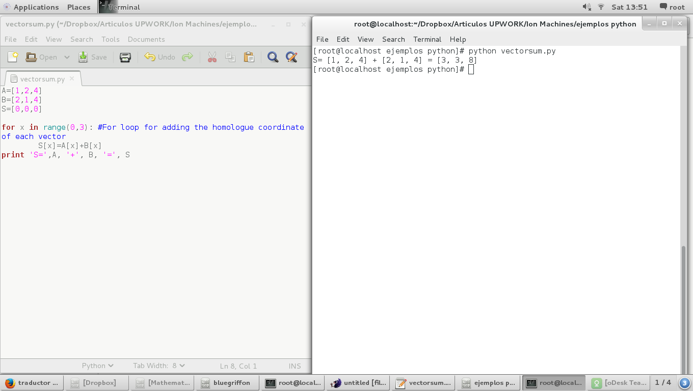
Product of a vector by a scalar
Given a vector:
A=[1,-2,3]
and a scalar:
scalar=-2
product vector by a scalar is defined as the scalar product of each coordinates of the vector:
for x in range(0,3):
    R[x]=scalar*A[x]
and the result is: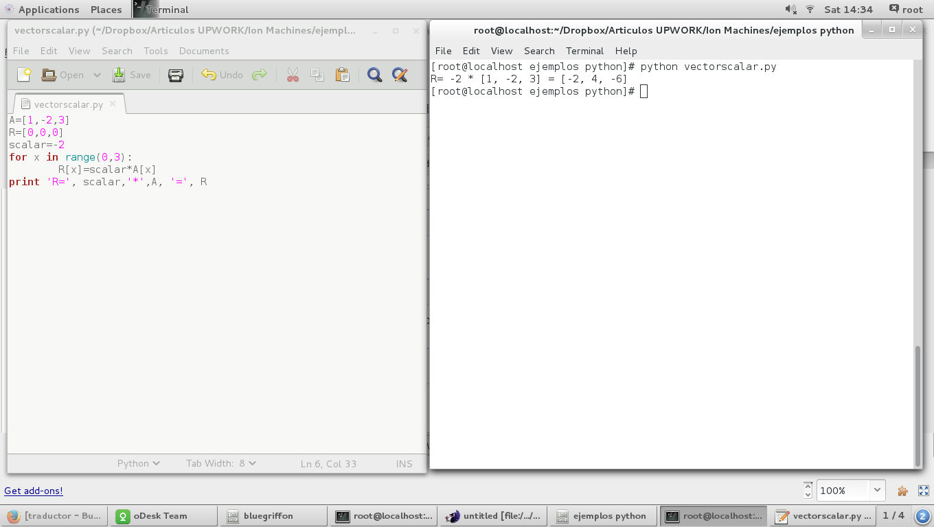
Unit Vector
Using the 'Magnitude of a vector' script we have:
V=[2, 2, 1]
U=[0,0,0]
modV=0
invmodV=0
import math
modV=math.sqrt(V[0]**2+V[1]**2+V[2]**2)
invmodV=1/modV
for x in range(0,3):
    U[x]=invmodV*V[x]
print 'U=',V,'/',modV,'=',U
and the result is: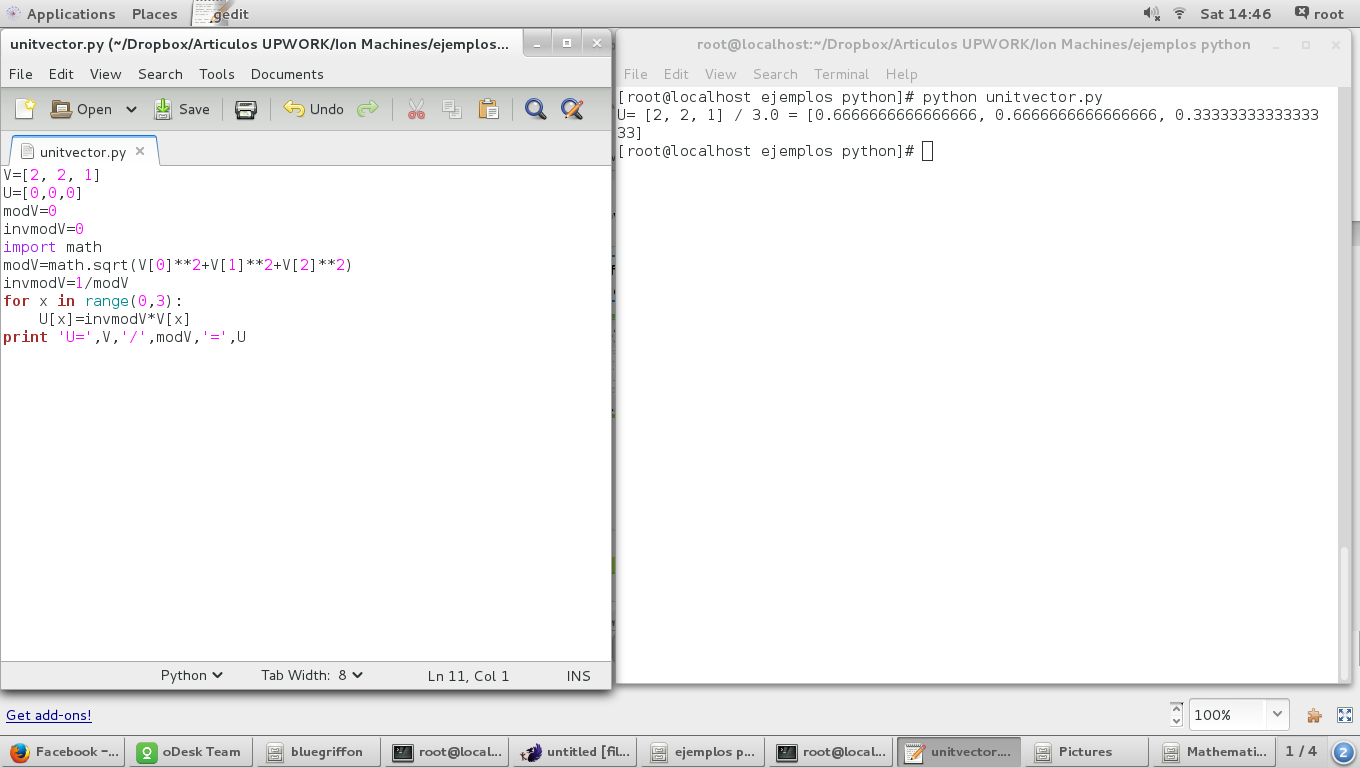
Linear Combination
Given three vectors , A, B and C , we can calculate the scalar values which, multiplied by B and C, respectively, results in the vector A. In other words, placing the vector A as a linear combination of the vectors B and C:
A=[7, 9, -8]
B=[1, 3, -2]
C=[-2, 0, 1]
A linear combination leads to a system of equations , 3 equations with 2 variables ( scalars ) if three vectors r3 , or 2 equations with 2 variables if they are two vectors in R3 , which can solve by applying a determinant of a matrix. Here we must make a point because of the data types handled by Python. In many cases when calculating the scalars involved in a linear combination, the result will have decimal places, which results in floating point operations. The numeric data types, handled by Python, are: Integer, Real, Long. So, we have to insert the coordinates of the vectors as Real data type, so these represent real numbers (floating point). We must know and understand some characteristics of the data type in Python:
- Integer take up less memory space than the Real type.
- Operations with Real are more slow than Integer.
Here we have the same vectors, but declared as Real type:
A=[7.0,9.0,-8.0]
B=[1.0,3.0,-2.0]
C=[-2.0,0.0,1.0]
So, with this we can swap the vectors and thus always have the system solution.
The first check we have to do is about whether there is coplanarity between the vectors or not, thus know whether or not there is a linear combination. For that, we are going to implement a determinant matrix:

det0=A[0]*(B[1]*C[2]-B[2]*C[1])-A[1]*(B[0]*C[2]-B[2]*C[0])+A[2]*(B[0]*C[1]-B[1]*C[0]) #Main Determinant involving all vectors
If this determinant is equal to zero (0) so there is a linear dependence between the vectors and we can continue calculating the scalars. As mentioned above, the system of equations have three equations with two variables, yielding a determined compatible system, for which we must take two of the three equations and solve scalar values, then check with the third equation, not taken before, if the previous scalars values solve it. If they don't solve this, then there is not a Linear Combination.

Here we have the complete code:
A=[7.0,9.0,-8.0]
B=[1.0,3.0,-2.0]
C=[-2.0,0.0,1.0]
det0=A[0]*(B[1]*C[2]-B[2]*C[1])-A[1]*(B[0]*C[2]-B[2]*C[0])+A[2]*(B[0]*C[1]-B[1]*C[0]) #Main Determinant involving all vectors
if det0==0:
    det1=B[0]*C[1]-B[1]*C[0] #First Determinant involving the first and second lines of the equations system
    if det1==0:
        det2=B[1]*C[2]-B[2]*C[1] #Second Determinant involving the second and third lines of the equations system
        if det2==0:
            print 'Linear Combination Unexistent'
        else:
            det3=A[1]*C[2]-A[2]*C[1]
            det4=B[1]*A[2]-B[2]*A[1]
            sc1=det3/det2
            sc2=det4/det2
            if sc1*B[0]+sc2*C[0]==A[0]:
                print 'Scalar 1 =', sc1, 'Scalar 2 =', sc2
                print A,'=',sc1,'*',B,'+',sc2,'*',C
            else:
                print 'Linear Combination Unexistent'
    else:
        det3=A[0]*C[1]-A[1]*C[0]
        det4=B[0]*A[1]-B[1]*A[0]
        sc1=det3/det1
        sc2=det4/det1

        if sc1*B[2]+sc2*C[2]==A[2]:
            print 'Scalar 1 =', sc1, 'Scalar 2 =', sc2
            print A,'=',sc1,'*',B,'+',sc2,'*',C
        else:
            print 'Linear Combination Unexistent'
else:
    print 'Linear Combination Unexistent'
And the result:
[root@localhost ejemplos python]# python lincomb.py
Scalar 1 = 3.0 Scalar 2 = -2.0
[7.0, 9.0, -8.0] = 3.0 * [1.0, 3.0, -2.0] + -2.0 * [-2.0, 0.0, 1.0]
[root@localhost ejemplos python]#
In conclusion, the basic vector algebra results in a series of operations involving linear systems of equations and / or simple arithmetic with real numbers. In another tutorial we will see how we can develop products with vectors, such as dot product, cross product or mixed product.

